WEEK 11 · 2026-03-23 ~ 29
Pic/Flip Particle Install
The PIC/FLIP particle system and the Bugis interior finally came together, with Week 10's audio driving particle behaviour. The project's title stopped being an intention and became a description of what was happening on the screen.
Until this week the project had been two parallel tracks. The PIC/FLIP particle system had existed since Week 8, running in a neutral test scene with no architectural context. The Bugis interior had existed since Week 10, a glass architecture built around the idea of religious coexistence, with no particles in it. Both halves worked. They had never met.
This week they met. The pond inside the Bugis interior started holding particles, the particles started responding to audio recorded in Bugis, and the thing I had been calling “Where Sounds Breathe” stopped being a title and started being a description of something happening on the screen.
PREPARING FOR INTEGRATION
The integration could not happen cleanly on top of the existing codebase. The simulation region, the interior models, and the render pipeline had each been set up assuming they would be used separately. Before the particles could move into the pond, a few pieces of infrastructure had to be rebuilt.
The first was the simulation region itself. Up to this point the PIC/FLIP simulation lived
inside a fixed box positioned at the origin of the world. That box was not where the
Bugis pond was. The SimBoxEditor was extended so that the Bugis interior could carry its
own simulation region definition, stored separately from the main scene
(bugis_sim_box_mesh.json). The editor itself gained a rotation mode and a PCA-based
alignment tool so the simulation region could be tilted to match the axes of the pond
mesh rather than the axes of the world.
Two smaller changes mattered. An OBJ cache was added so interior meshes only had to be parsed once rather than every time the interior was entered, which cut the re-entry load time from seconds to nearly zero. And the gizmo picking was updated to account for object scale, so the larger interior models (the city block, the religious buildings) could be selected and moved without having to zoom in on them.
None of this is visible in the final experience. The visitor never sees the simulation region overlay or the gizmo. But without this week of preparation the integration would have been fighting the architecture of the existing code the whole way.
THE INTEGRATION
The particles entered the pond on March 26th. The first visible result was strange. Particles appeared at the correct location, but the shape of the pond was not guiding the fluid the way I expected. The simulation region was a rectangular box, and the pond mesh was a curved, organic shape inside it. Particles outside the pond mesh but inside the region box were still being simulated, which meant fluid existed in places there was no pond.
The fix was two-part. The simulation world origin was moved from a fixed world position to the corner of the pond’s axis-aligned bounding box, so the simulation grid covered only the region that actually mattered. This let the SDF (signed distance field) resolution focus on the pond interior rather than wasting precision on empty space around it. And the depth occlusion pass was rewritten to compare particle view-space Z against the interior’s depth texture in linear space, so particles that were geometrically behind the pond rim or the surrounding glass architecture were correctly hidden.
A small z-fighting issue between the pond surface and the floor water beneath it was
solved with polygon_offset on the floor, which pushes the floor’s depth slightly further
from the camera without changing its appearance. Small detail. It had been making the
water surface flicker for two days before I named the cause.
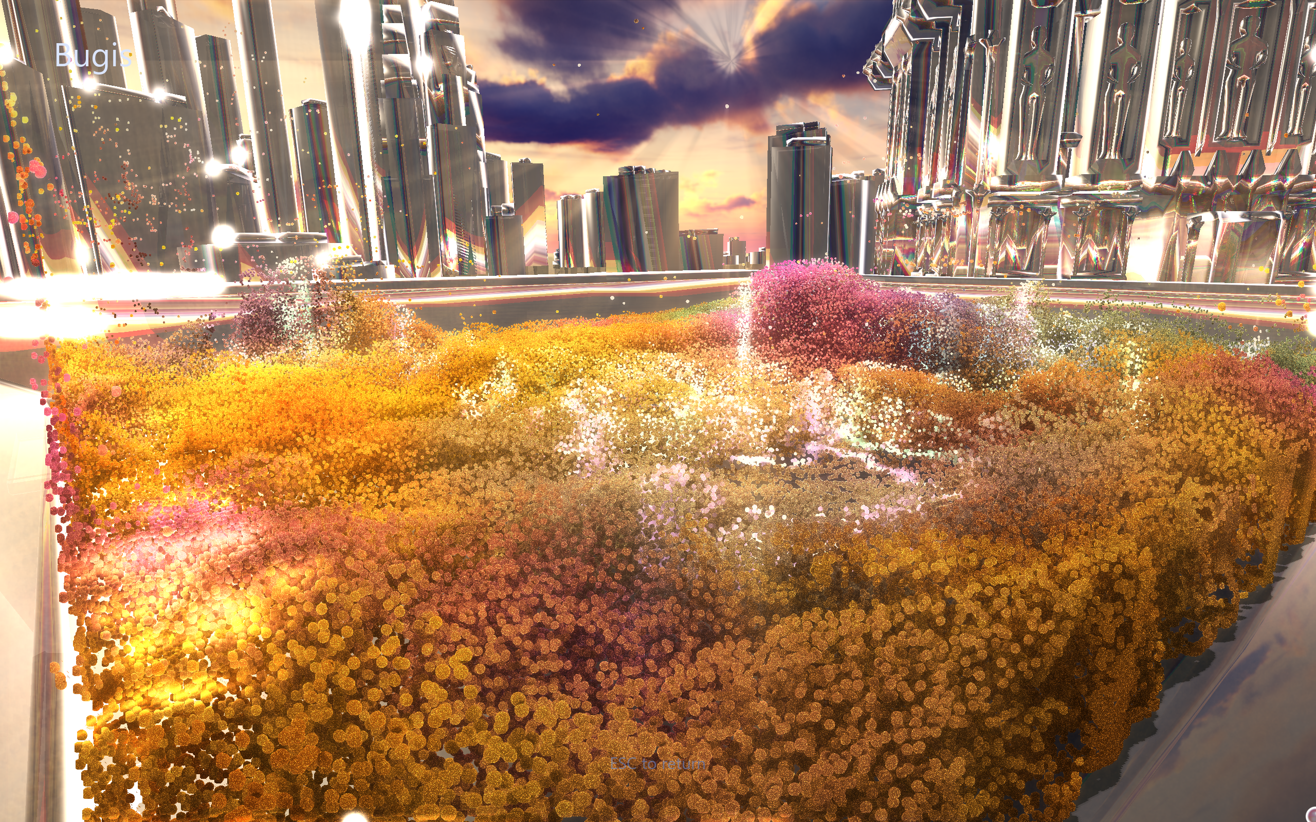
The first integrated frame. Glass city on the horizon, the pond's particle bed sitting in front of it, the two halves of the project finally in the same scene.
Once the particles were behaving correctly inside the pond, the scale problem became the next issue. Fifty thousand particles had been fine in the empty test scene of Week 8. The Bugis interior was carrying hundreds of thousands of triangles of glass architecture, an HDRI skybox, volumetric fog, and a reflected floor. Rendering five hundred thousand particles on top of all of this with the existing icosphere geometry dropped the frame rate below what was usable.
The solution was billboard rendering. Instead of each particle being a small sphere made of 320 triangles, each particle became a camera-facing quad made of 2 triangles. The fragment shader for the quad does a ray-sphere intersection per pixel so the particle still looks spherical and shadows correctly, but the vertex load is about 160 times lighter. This change alone brought the frame rate back up without visibly changing what was on screen.
The integration in motion. Billboard rendering, correct depth occlusion, the fluid holding its shape inside the pond mesh.
AUDIO MEETS PARTICLE
The integration on its own was a technical milestone. The work that made it the point of the project was what happened next. The thirteen recordings captured in Week 10 had been sitting as audio files. This week they started driving the particle system.
The setup is an audio_analyzer module that plays a recording while running an FFT on it
every frame, extracting three frequency bands (bass, mids, treble) and a combined energy
level. These four values are uploaded to the GPU every frame as uniforms. The particle
compute shader reads them and uses them to apply forces to the fluid.
Marina Jung Morgan’s advice from Week 10 was in the back of my head through all of this:
The force design followed that principle. Large-scale motion is driven by the ambient energy of the recording. Small, readable details appear on top of the ambient motion. Six different forces are blended together to produce the final behaviour of the fluid, and while all six contribute, a few of them are the ones a viewer actually notices.
-
Water droplet ripples on the treble
Short, high-frequency content in the recording produces localised ripples on the surface of the fluid. Each ripple is a small force origin that pushes the fluid outward briefly and then fades. Twelve such ripple origins are active at any moment, with their positions rehashed every third of a second, so the surface always has small detail events happening somewhere but never in a predictable pattern. This is how the symbolic details from Marina’s framing become visible. A crosswalk beep in the recording becomes a ripple in the pond.
-
Radial pulses on the bass
Bass content drives larger, slower pulses. Five pulse centres are distributed across the pond, each pushing fluid outward when a bass frequency peaks. Unlike the treble ripples, these pulses are felt more than seen. The fluid bulges and settles. The motion reads as weight rather than as event. When the recording has a sustained low rumble, the surface of the fluid has a continuous breathing motion.
-
Surface waves on the ambient bed
The ambient energy of the recording, the thing Marina said was what made a place specific, drives a continuous low-frequency surface wave. This is not an event. It is the constant. It is always happening, at different amplitudes depending on how loud the ambient is in the current moment of the recording. This is the force that gives each recording its baseline character. The Kwan Im temple recording has a different waveform than the Hawker Center recording because their ambients are different, and the fluid’s baseline shape reflects that difference.
Two additional forces (a slow vortex that activates when bass and mids are simultaneously strong, and a full-world explosion that only fires when combined energy exceeds a high threshold) sit on top of the three above. They are rare enough that they feel like punctuation rather than rhythm.
The colour of the fluid also responds to the audio, but the mapping is spatial rather than global. Instead of the entire fluid turning red when the bass is high, bass creates warm colour zones that drift across the pond in a sine pattern. Mids do the same in a teal-green band at a different frequency. Treble produces bright sparkle points at hash-based random positions that change each frame. The result is that the fluid looks different in different parts of the pond at the same moment, and the pattern evolves over time as the audio evolves.
Two frames from the integrated version show what this looks like at different states of a Bugis recording.
Audio meeting particle. Ambient bed driving the slow surface wave, bass pulsing the colour zones, treble sparking ripples on top.
One thing that surprised me during development was how much the normalisation of the FFT mattered. Ambient recordings have much lower energy than music, and the default FFT scaling produced no visible reaction to most of the Bugis recordings. The energies had to be boosted aggressively (dividing the raw energy by 8 for bass, 4 for mids, 2 for treble) to bring the response into a useful visual range. Without this, the Kwan Im temple recording looked like the fluid was almost completely still. With it, the same recording drives clear, readable motion.
FINAL RESULT · END-OF-WEEK STATE